Your halftone is lying about its midtones
Notes from building a Risograph simulator that had to be exact.
A halftone filter and a printed halftone are not the same object. The filter puts a pattern of dots over a photograph. A press separates the photograph into plates, screens each one, and prints them in sequence onto a sheet that is neither flat nor uniformly absorbent. Almost everything interesting happens in the gap between those two descriptions.
I spent a while closing that gap for tone +, a Risograph simulator for iOS. The engine is about five thousand lines, has no third-party dependencies, and ships in 3.2 MB. What follows is the part of it that surprised me.
1. Separation is a least-squares problem with 27 corners
The obvious way to make a two-colour print out of a photograph is to map luminance onto a colour ramp. That is what a duotone filter does, and it is why duotone filters look like filters: it throws away the photograph’s chroma and then invents some.
A press does something different. It lays down N inks whose transmittances multiply. Written in optical density — the log of the reciprocal of transmittance — multiplication becomes addition:
D(x) = Σᵢ aᵢ(x) · Dᵢ with each aᵢ ∈ [0, 1]
where Dᵢ is the density of ink i at full coverage and aᵢ(x) is how much
of it lands at pixel x. So recovering the plates from a photograph is a
linear least-squares problem in at most three unknowns, subject to a box
constraint. Not a colour mapping — a fit.
The box constraint is what makes it awkward. Unconstrained least squares has a
one-line solution; add 0 ≤ aᵢ ≤ 1 and the textbook answer is to iterate:
projected gradient, active set, NNLS. All of which need convergence tuning, and
all of which are miserable to vectorise over a million pixels.
But look at the dimension. A box-constrained convex quadratic attains its
optimum on some face of the box, and each ink is in one of three states —
pinned to 0, pinned to 1, or free. With n ≤ 3 that is 3ⁿ ≤ 27 faces total.
Twenty-seven is a small number. Each face has a closed-form minimiser, and — this is the part that makes it practical — the matrices involved depend only on the ink set, not on the pixel. So they are computed once for the whole image, every face is evaluated for every pixel simultaneously as a handful of matrix multiplies, and the answer is the best feasible one.
No iteration. No convergence criterion. No tolerance parameter that is wrong on somebody’s photograph. The exact global optimum, in closed form, vectorised.
There is a small trick that keeps it clean. Rather than solving a k×k system
on just the free indices of each face, each face is stored as a full n×n
affine map with the pinned coordinates folded into the offset vector. That
wastes a few multiplies and saves all the per-face fancy indexing, which at a
million pixels a frame costs more than the arithmetic does. It has a pleasant
side effect: the pinned coordinates come out as exactly 0.0 or 1.0, so a
blanket “is every component in [0,1]?” doubles as the feasibility test for
the free ones.
I verified it against a dense grid search over the box. It never loses.
2. The screen that drifts
Here is the bug I did not expect to find, and which I now suspect is in a great many halftone implementations.
A halftone screen is a threshold function. You have a cell, you have a
requested coverage c ∈ [0,1], and you need the dot in that cell to occupy
fraction c of its area. The usual approach is to write a smooth analytic
threshold field over the cell — a cosine, a distance function, something with a
convenient closed form — and threshold it at c.
The trouble is that thresholding a shape field at c does not generally ink
c of the cell. It inks whatever fraction of the cell has field value below
c, which is only equal to c if the field’s value histogram happens to be
uniform. For a round dot it is not. For an elliptical dot it is really not. So
the printed area only approximately tracks the requested tone, and the error is
largest exactly where the eye is most sensitive: the midtones.
You can paper over this with a per-shape calibration curve, tuned by hand until the greys look right. That is a magic number standing in for a missing idea.
The fix is to stop guessing what the threshold produces and compute it. Sample the dot’s shape over one cell, reduce it to a value histogram, and you have the exact map from threshold to inked fraction — its cumulative distribution. Invert that, and you have the threshold that produces any requested coverage, exactly. Once per shape, cached.
The result reproduces requested coverage to within a fraction of a percent at every level, for every dot shape and every ruling, with no per-shape calibration at all. Change the dot from round to cross and the tone does not shift.
Fold the anti-aliasing into the same calculation. This is what makes it correct at the extremes. The dot’s edge is a ramp rather than a step, and through the midtones a symmetric ramp cancels itself — as much ink gained on the inside as lost on the outside. At 0% and 100% it does not cancel, because one half of the ramp is clipped away by the cell boundary. Handle the edge separately from the area and you get a phantom dot in every cell of bare paper and a pinhole in every solid. Compute the histogram of the anti-aliased field, and both disappear, because the thing you inverted was the truth.
3. Overprint is not alpha blending
When two plates overlap, what colour is the paper?
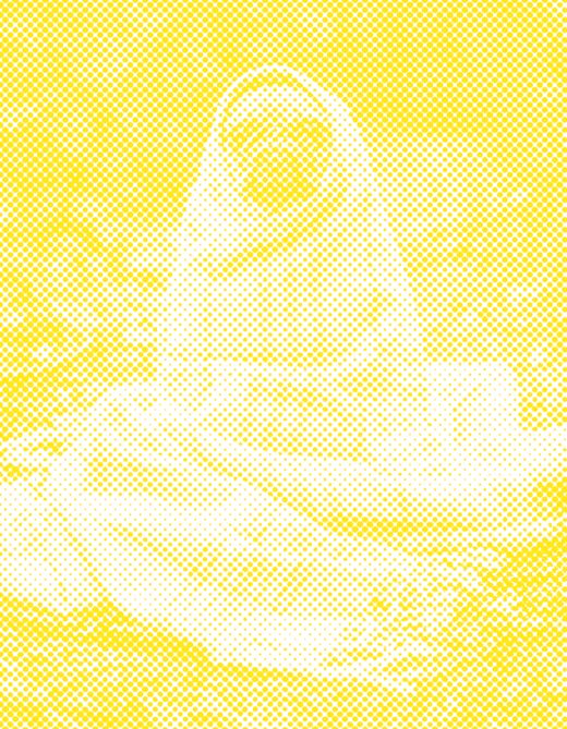
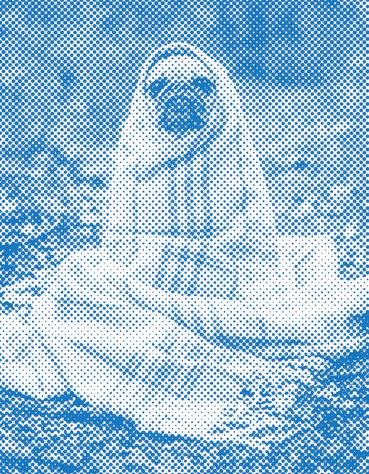
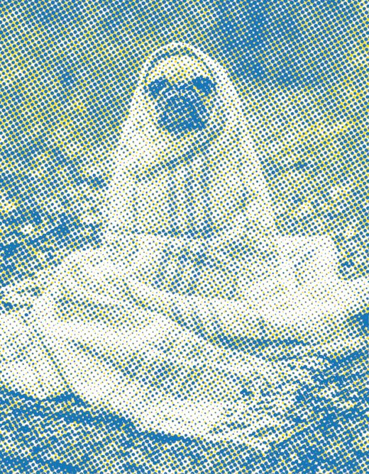
Alpha blending says: interpolate. Which gives, for a red plate over a blue one, something close to their average — a muddy grey-purple that looks like neither ink and like no print anyone has ever held.
Ink is not paint laid on a surface. It is a filter that light passes through twice, on the way in and on the way back out. So a plate’s contribution is multiplicative against whatever is already on the sheet:
R ← R · T
But real Risograph ink is not perfectly transparent either. It is a pigment layer with some hiding power — that is what an opacity control actually describes. Interpolating the substrate towards white before applying the filter gives both ends from one expression:
R ← T · lerp(R, white, opacity)
At opacity = 0 the ink is a pure multiply and picks up everything printed
underneath. At opacity = 1 it shows its own colour regardless of what is
beneath it. In between it does the thing real ink does.
That single lerp is why red over blue gives a plausible dark purple instead
of mud. It is three operations and it carries more of the “this looks like a
print” feeling than anything else in the pipeline.
4. One noise field, two effects
Paper is where I expected to spend the least effort and ended up spending the most.
The obvious model is: paper has a texture, so multiply a noise field over the final image. This gets you a photograph with grain on it.
What actually separates a photo with a halftone on it from a photograph of a print is that the sheet’s unevenness does two different things at once:
- The surface does not reflect light uniformly. (This is the effect everyone models.)
- That same surface does not accept ink uniformly. Fibres standing proud get inked; pits get missed.
The second one is the one that matters, and it has to come from the same noise field as the first, because in a real sheet it is the same fibres doing both. Model them independently and you get two uncorrelated grains that read as noise. Drive them from one field and you get mottle — the patchiness that stops large flat areas looking like they were poured out of a paint bucket.
Feature sizes are held in reference pixels and scaled by the render scale, so a 900px preview and a 4000px export show grain of the same visual size. A preview whose grain is four times too coarse is not a preview.
5. “47 lpi” is not a number
Lines per inch is a ratio. It says nothing until you say how many inches the sheet is, and a digital image does not have inches.
This is not pedantry — it is the difference between a preview and an export agreeing or not. Get it wrong and your on-screen proof shows a different screen from the file you save, which is the one bug in this whole domain that users will actually notice.
So I measured. Take real output, take its Fourier transform, and the screen announces itself: a periodic structure shows up as a pair of peaks whose distance from the origin is the ruling and whose orientation is the angle. Read them off, count the dots across the sheet, and divide by the stated lpi. The answer came out at a 3.44-inch sheet — 45°, 47 lpi, about 162 dots across.
Now lpi means something. Ruling is defined against a physical sheet size, the render scale falls out of the pixel dimensions, and a preview and a full-resolution export show an identical screen because they are both screens on the same 3.44-inch sheet.
6. Two implementations, on purpose
The engine exists twice: once in Python with NumPy, once in Swift. Not as a port — as a cross-check.
Numerical code is uniquely good at being confidently wrong. It runs, it produces an image, the image looks plausible, and the midtones are off by four percent. Tests help, but a test is only as good as the property you thought to assert.
Two independent implementations of the same mathematics, compared numerically, catch a whole category of error that neither one’s own test suite will: the kind where you asserted the wrong thing in both places but implemented it differently. When the Swift screen and the NumPy screen agree to within tolerance at every coverage level, for every shape, that agreement means something no single implementation’s tests can mean.
It is expensive. I would do it again.
Postscript: measure your build configuration
Swift’s debug configuration is -Onone: no inlining, no generic
specialisation, bounds and overflow checks retained. This engine is per-pixel
numeric loops over millions of pixels — exactly the code that lives or dies on
optimisation.
Measured, in this project: about 80× slower.
The interesting part is how it presents. Rendering runs off the main actor, so the UI stays perfectly responsive. Nothing hangs. Nothing beachballs. A photo goes in and no print ever comes out. It does not look like a slow app. It looks like a broken one, and I lost a debugging session to it before I thought to check which configuration was on the device.